Weather, routing and corrected time
A start-window range, route comparison, forecast-policy mean and corrected-time margin answer different questions. They cannot be added.
| Weather and route comparison | Hours | 95 % interval |
|---|---|---|
| Best versus worst scheduled start, same boat | 29.2 | [18.5, 47.7] |
| Division winner versus its actual rivals | +0.02 | [−1.12, +1.16] |
| Speed-band median line versus hindsight | −0.43 | [−9.12, +8.26] |
| Whole-fleet median line versus hindsight, Transpac | +5.00 | [−0.53, +10.54] |
The first is a best-to-worst range. The others progressively replace real rivals with composite lines and hindsight, so the broader comparisons control less.
| Forecast comparison | Hours | 95 % interval |
|---|---|---|
| Ensemble hedge, per eligible race-month cycle | +1.10 | [+0.41, +1.92] |
| Observed-extreme missing-outcome sensitivity | +0.62 … +2.06 | [−0.07, +3.35] |
The sensitivity values are scenarios, not bounds. At 8.9 knots, +1.10 h is about 10 nautical miles.
| Corrected-time comparison | Hours | Interval |
|---|---|---|
| Whole division, fastest to slowest | 40.8 | [31.7, 47.6] |
| First to the division median | 12.6 | [11.2, 14.3] |
| First to second | 4.81 | [3.60, 5.89] |
| Race-relevant sister-ship spread | 4.36 | n/a |
| Full ORC sister-ship spread | 3.80 | n/a |
| One boat's year-to-year certificate change | 0.70 | n/a |
Certificate hours translate observed fractional differences onto a reference passage. They are not estimates of rating error.
In the paper. See Table 1; §§5.3–5.4 for route comparisons; §§6.1–6.4 for scoring, certificates and starts; and §7.1 with Table 14 for the forecast policy.
Sustained route separation
The first strategic question is physical: how far north can the boat go before the shorter course meets the light air under the High? A northern line saves distance. A southern line usually keeps more wind. The ensemble offers several plausible answers before the start.
To measure when those answers become distinct, we scan the candidate routes westward. A crossing only counts when their north–south spread remains above the chosen threshold through 150°W. Routes can split around weather and later rejoin, so a first divergence alone does not meet this definition.
With a 30-nautical-mile threshold, the median K = 5 forecast cycle reaches sustained separation 199 nm from the start. The K = 8 analysis reaches it at 147 nm. Separation is found in 99 of 100 K = 5 cycles and all 100 K = 8 cycles. We report the cluster counts separately because they are two analyses of the same forecast cycles, not two independent samples.
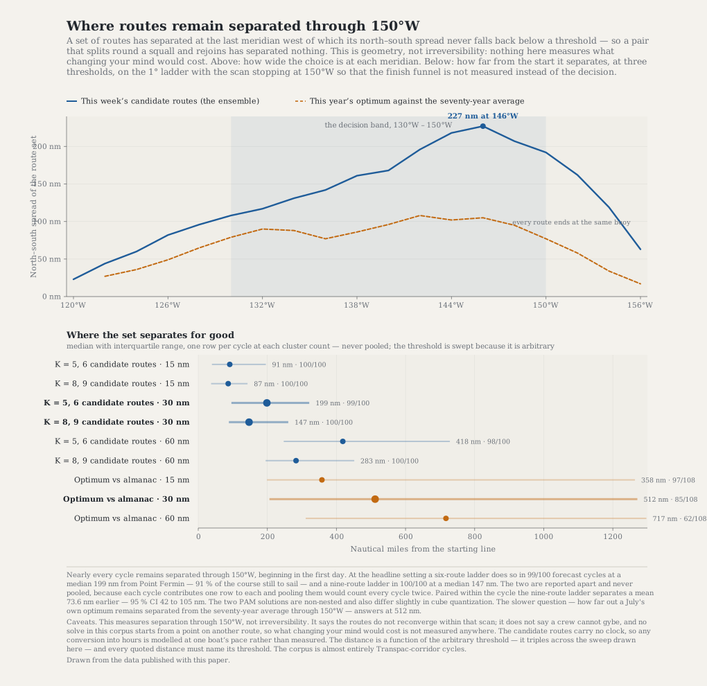
The exact distance depends on the rule. At a 15 nm threshold the median is about 90 miles; at 60 nm it is about 400. A forward scan gives 154 nm. The candidates' median maximum spread is 227 nm at 146°W. Those checks support one qualitative result: the route set acquires and maintains substantial lateral separation early in the passage.
That result does not locate a point of no return. The scan stops at 150°W, before the Honolulu finish funnel. It does not re-route a boat after it crosses from one candidate to another. It therefore measures neither switching cost, replanning cost nor practical irreversibility. It also does not show that everything after the first day is boat speed.
Compare the north and south alternatives before the gun and during the first day, when they are still near one another. Later course changes may remain possible; this study has not measured their cost.
In the paper. See §4.2 and Table 2 for the result, §3.9 for the four choices in the separation definition, and §9.7 for the limit on switching and irreversibility.
Winners against their own divisions
Across 78 divisions, corrected-time winners are compared with the boats that shared their start and weather. Each track is replayed individually on the same hypothetical boat.
Winners do not occupy a detected special lane. Their latitude differs from their division median by −0.5 nm [−11.1, +10.2], and their closeness to the hindsight optimum by −2.4 nm [−9.6, +4.8]. Their replay difference is +0.02 h [−1.12, +1.16].
Their recorded ground tracks are shorter more often: −12.0 nm [−22.6, −1.5] on average. When the tracks are reduced to the same meridian grid, that difference disappears, locating it between the slices, in gybes, steering changes or local-weather deviations that sparse trackers cannot resolve. Longer tracks also tend to place worse, with pooled Spearman ρ = +0.221.
Modeled current does not explain the result. Winners sail 10.7 nm less through the water, while their current assist differs from rivals by −0.72 nm [−3.77, +2.33].
These are observational associations. A boat may sail fewer miles because it is already positioned in the right weather; the archive does not establish that shorter distance caused the win.
In the paper. See §5.3 and Table 6.
The best route depends on the boat
A route is fast for a particular polar in a particular week's weather. Across the paired Transpac panel, the faster boats remain within about 12 nm of the canonical route, while the Santa Cruz 50, J/121, J/122 and Cal 40 run 29.9–58.1 nm north through the decision band. The panel's spread reaches 114 nm at 138°W.
Changing only the canonical polar's deep-running speed shows why. Reducing it by 5 % moves the optimum 25.0 nm north [+7.6, +42.4]; increasing it by 5 % moves the route 17.6 nm south [−33.1, −2.0]. Comparable reaching and upwind changes alter elapsed time without a detected latitude shift.
The perturbation changes one part of one polar and cannot show that deep-running performance causes the full between-boat ordering. Verify the boat's polar and use similar-speed boats as visual references; the middle of a mixed fleet is not neutral.
In the paper. See §6.5, Tables 12–13 and Figure 7.
What the certificate can change
Under time-on-time scoring, 0.001 of coefficient is worth about a quarter hour on these passages. First and second finish a median 4.81 h [3.60, 5.89] apart, and a change of 19.0 thousandths [14.9, 26.4] would flip the median division result.
Matched sister ships differ by 1.60 % [1.50, 1.69] in GPH. Designs sailed in these races give a similar 1.83 % [1.53, 2.24]. Their point conversions are 3.80 and 4.36 corrected hours on the reference passage. One boat's de-trended year-to-year movement is much smaller: 0.29 % [0.285, 0.300], about 0.70 h.
Sister-ship scatter combines real configuration and certificate differences. Sails, propeller, keel, loading and displacement can legitimately differ, so this is not certificate error or evidence of gaming. The conversion from ORC to the race rules also assumes comparable fractional scatter, which this archive cannot test.
Winners do not cluster at one end of the rating band. Their median position is 0.500 [0.375, 0.600]. The data support checking why sister ships rate differently; they do not support chasing one end of the band as a general winning strategy.
In the paper. See §§6.1–6.3 and Tables 8–10.
What the ensemble decision was worth
One deterministic forecast gives one route. Fifty ensemble members give several plausible weather outcomes and candidate routes. The tested rule chooses among those routes by limiting expected loss in the worst third of member outcomes, subject to a three per cent forecast-time cost cap. It may keep the deterministic route; that decision contributes zero.
A positive gain means the selected route was faster than the deterministic route when both were verified in ERA5. This is a comparison among routes generated from the forecast, not against an unrestricted hindsight optimum.
Across 60 of 63 eligible June–July cycles, mean gain is +1.10 hours per cycle [+0.41, +1.92]. At 8.9 knots that is about 10 nautical miles.
Three cycles contain no scoreable firing. Replacing missing outcomes with the worst observed gain gives +0.62 h [−0.07, +1.36]; replacing them with zero gives +1.03 h [+0.39, +1.76]; and replacing them with the best observed gain gives +2.06 h [+1.00, +3.35]. These are observed-extreme sensitivity scenarios, not bounds. The pessimistic interval includes zero.
The worst observed loss is −5.15 h. The rule can choose only from its candidate set, and the forecast distribution may miss the weather. The historical mean therefore provides no guarantee of future gains.
In the paper. See §7.1 and Table 14 for the policy estimate and missing-outcome sensitivity, and §7.2 for the onboard interpretation.
Climate trends and departure dates
Hold the course, boat and solver fixed and change only the historical weather. Over the satellite era, the fitted change in optimum elapsed time is +10.1 h [−9, +29]. No route metric has a detected trend at the precision of this archive. That does not show that the Pacific climate is fixed; it says this navigational integral cannot separate a smaller drift from year-to-year variation.
Departure timing matters much more. Departures five days apart differ by 26.4 h on average. Across 6–16 July, the best-to-worst range averages 45.0 h. A seasonal mean can describe a July, but it cannot choose the weather of one start.
Pressure is useful for describing the High but not for locating the route. Out of sample, the pressure rule has 117.6 nm RMSE, against 77.3 nm for latitude. The flank is shallow, about 84 nm per hPa, so a small pressure difference spans many miles.
Use climatology as background, then solve the actual forecast and start window. A fixed pressure target does not replace that work.
In the paper. See §§4.3–4.4 and Tables 3–4.
Pacific Cup 2026 and race preparation
The 2026 Pacific Cup shows one limit clearly. Before the second start, all fifty ensemble routes crossed 142°W between 26.54°N and 29.58°N. The later ERA5 hindsight optimum crossed at 31.05°N, while the fleet median crossed at 28.82°N, a 133.7 nm fleet-to-hindsight gap. No selection rule restricted to those candidates could have chosen the northern route.
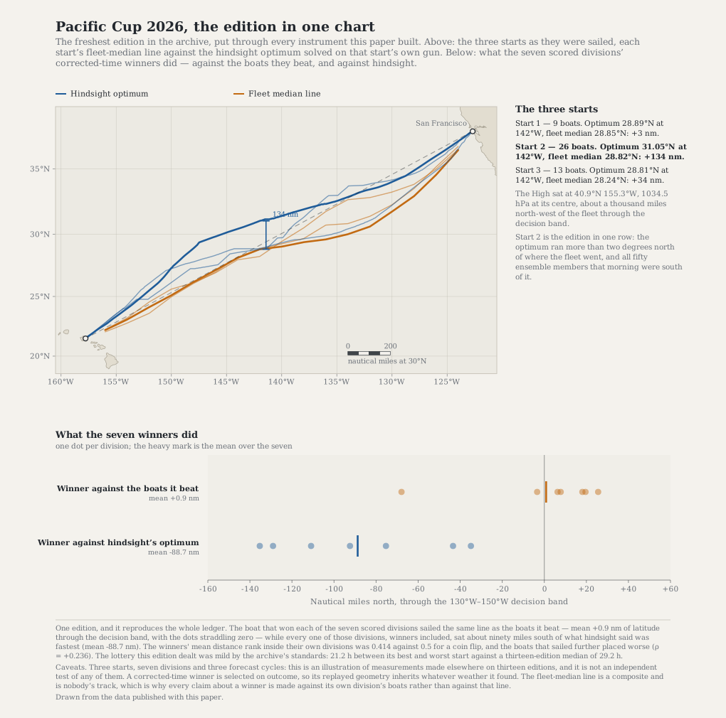
Figure 3 — Pacific Cup 2026, the edition in one chart. The chart carries the three starts of one race: the orange lines are where the middle of each start’s fleet actually went, the blue lines are the hindsight optimum from that same gun, and the bracket on 142°W is the gap between them for the second start. Below, each dot is one scored division: the top row is how far north or south of its own rivals the winner sailed, the bottom row is how far it was from hindsight’s optimum, and the heavy mark is the mean of the seven. This edition illustrates measurements made across the larger archive; it is not an independent test. Across these seven qualifying divisions, the mean winner-versus-rivals latitude difference was +0.9 nm. Start 2’s hindsight optimum ran more than two degrees north of its fleet median, and every forecast member for that start lay south of the hindsight optimum.
That does not show that the fleet ignored a forecast or chose badly. The archive does not know which products navigators used, and the hindsight route had information they did not. It shows that the forecast distribution can miss the later answer on one side.
Race preparation checklist
Before the race
- Check the certificate and compare changes with the typical 4.81 h first-to-second margin.
- Verify the polar, especially deep-running speed; plausible changes move the computed route by tens of miles.
- Compare with boats of similar speed rather than the middle of a mixed fleet.
When choosing a route
- Solve the actual start window; five days changes the same boat by 26.4 h on average.
- Inspect candidate routes and downside, not only the deterministic route or a grid-cell spread.
- Treat sustained separation through 150°W as geometry, not a point of no return.
After the race
- Review distance, latitude, speed and weather separately. Winners record shorter tracks more often, but the archive does not establish why.
- Keep start-day ranges, forecast-cycle gains and corrected-time margins in separate columns.
In the paper. See §8, Table 15 and Figure 9 for the 2026 example; §§4–7 contain the archive-wide comparisons.